Veusz has long existed as a 2D-only plotting GUI application and library. From version 3, Veusz now supports several types of 3D plots. As with previous versions of Veusz, plots are flexibly built out of a number of plotting widgets, allowing several 3D graphs to occupy a 3D space. Veusz renders the 3D output in vector format, which means the full quality of the plot is retained when scaling. Currently implemented plot types include 3D points, line, data surface, functional surface, functional line and volume plots. This page is a guide for how 3D plotting works.
3D plotting in Veusz uses the same widget scheme as 2D plotting, but first the user should add a 3D scene widget (scene3d) to the page. Alternatively, the user can make a new document with a 3D graph (see the File, New menu). The scene is a 3D volume which is viewed on the page. All 3D widgets must be placed within a scene or its subwidgets. The scene controls the viewing angle to the 3D widgets and the distance of the origin of the graph to the viewer. See Rendering below for more details about how the rendering works.
By default the view of the scene is automatically scaled up to fill the bounding box of the scene3d widget. This is controlled by the “Size” setting of the scene. The default “Auto” value can be changed to be a number which gives the scaling. Fixed scales can be useful to give a consistent plot size which does not vary by viewing angle, which is helpful to create animations.
The viewing angle is specified by the user as three rotation angles in degrees around three axes. These axes are not the axes of any graphs. The z axis lies along the line of sight through the 3D origin. The x axis lies horizontally on the page through the 3D origin. The y axis lies vertically on the page through that origin.
The origin is the default location of a 3D graph. It lies at a distance to the viewer controlled by the “Distance” setting of the graph, where the default graph size has a size of 1. When the distance is smaller, the effect of perspective is greater. By increasing the distance, the graph can becomes close to an isometric projection. With the default automatic scaling, the size on the page does not change.
| Distance 5 | Distance 50 |
|---|---|
 |
 |
The colour of solid surfaces and lines is determined by their intrinsic colour, plus an additive effect of lighting. The angle from the light source, the light source colour and intensity and the surface reflectively are used to calculate an additional colour contribution to the surface. Up to three light sources can be defined in the scene. The position of the light sources are defined relative to the camera or viewer, not the graph. Positive values for X, Y and Z positions lie to the right, upwards and towards the graph, respectively.
| Light angle 1 | Light angle 2 |
|---|---|
 |
 |
Normally in Veusz, sizes of objects (e.g. plot markers) are given in physical units. This makes less sense for a 3D plot as sizes can depend on distance. In a 3D graph sizes of plotting markers and line widths are given in 1/1000 of the graph bounding box maximum dimension.
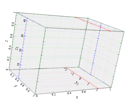
One or more 3D graph widgets are placed in the scene3d widget. The default location in 3D space of this widget is the origin 0,0,0. If you want to use more than one, they currently must be manually positioned. Each 3D graph widget also has a size in each dimension (by default 1,1,1). Currently, if the graph size overlaps the viewer/camera, then the output will look strange. The graph has formatting settings for its surrounding lines and the surface of the rear faces.
| Multiple 3D graph widgets in a single scene |
|---|
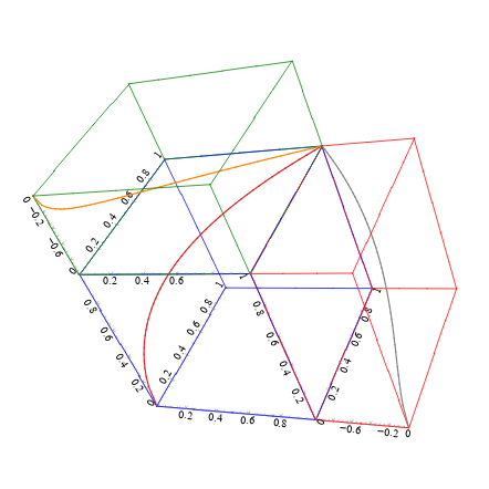 |
The 3D graph contains three or more 3D axis (axis3d) widgets, with at least one for each dimension. This is analogous to the standard 2D graph with two or more axis widgets. The widget has options for the axis label, tick labels, tick marks and grid lines (which appear on the outside of the 3D cube). An axis can be switched between linear and logarithmic mode. Scalings can be applied to the data values plotted in that dimension or to the axis labels.
Similarly to the 2D axis, the 3D axis has positions which allow it to appear mid-way down the cube in the other dimensions. This allows the user to add multiple non-overlapping axes for each dimension.
| Multiple 3D axis widgets in a single graph |
|---|
 |
Similarly to the 2D graph, the 3D graph contains one or more plotters. Unlike the 2D graph, the ordering does not matter. We list the various plotter types here.
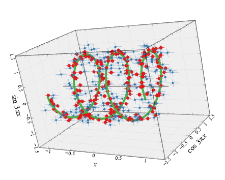
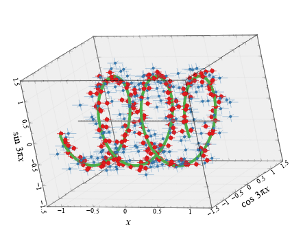
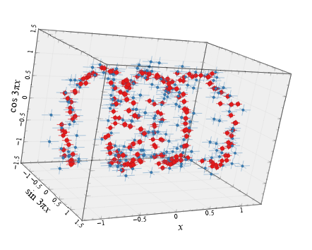
This plotter takes three 1D datasets giving X, Y and Z values. Points are plotted at each position. Optionally, a line connecting the points is plotted. A fourth dataset (Size) can be provided which scales the size of each point. Another dataset can be provided to colour the markers or the line (a minimum, maximum and scale can be set to give the scaling). The colour map used for plotting is provided under the formatting settings (for marker fill and line).
The point plotter also supports error bars in each dimension, similarly to the 2D plot.
| 3D point plotting example |
|---|
 |
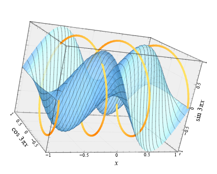
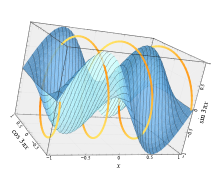
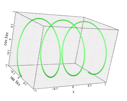
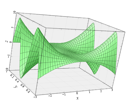
Plots either a functional line in 3D space or a functional surface. The type of plot is given by the mode parameter. In the case of the line, the x,y,z coordinates can be specified as a function of t, where t goes from 0 to 1, or by giving functions for two of the coordinates as a function of the other. For a surface, the value for x, y or z is given as a function of the other two. In addition, a function returning 0 to 1 can be provided for the colour, which specifies the colour map value for the surface at each position or the line col-or. For a 2D surface, the grid lines or surface fill can be hidden or shown. There are also settings giving the number of function evaluations to compute in each direction for a surface, or in one direction for a line.
| 3d line function | 3d surface function |
|---|---|
 |
 |
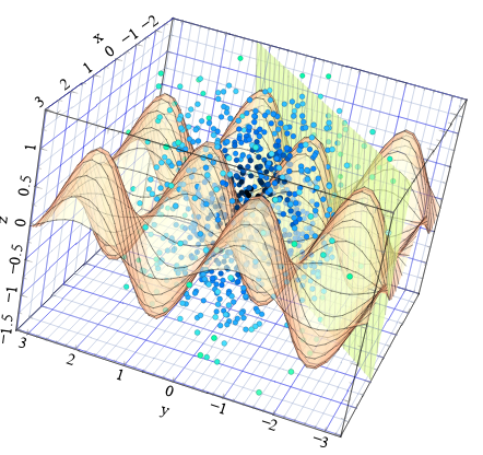
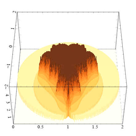
Plots a two dimensional surface from data values. The user should provide a 2D dataset for the height of a surface. The x, y or z axis for the height and other directions can be chosen. A second 2D dataset can be provided for the colour of the surface at each point. Note that the coordinate of the 2D dataset lies at the centre of each 2D grid point. The height of the grid at the edge is calculated by linear interpolation. Normally the grid is surrounded by four lines and the surface by two triangles. If a high resolution option is enabled, the each grid point is surrounded by eight lines and the surface drawn by eight triangles.
| 3D surface plotting example |
|---|
 |
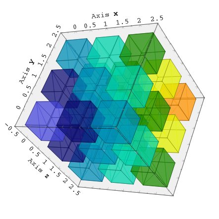
Plots 3D volumes drawn as rectangular cubes. In this widget, for a volume described by A×B×C values, then the user should provide four datasets, each containing up to A×B×C values (there can be holes in the representation). Three of the datasets give coordinates of the centers of the 3D cells and the fourth the colour of the cell. An example set of datasets would be X=(0,0,0,0,1,1,1,1), Y=(0,0,1,1,0,0,1,1), Z=(0,1,0,1,0,1,0,1), color=(0.1,0.2,0.3,0.4,0.3,0.2,0.1,0). Additionally, the user can provide a transparency dataset, which can be useful for showing or hiding parts of the 3D space.
| 3D volume example |
|---|
 |
Note that Veusz does not use a standard method for making 3D output (e.g. OpenGL). This is so Veusz can produce vector rather than bitmap or raster output. A future version could also support OpenGL for speed.
In detail, Veusz renders the 3D scene by making a list of lines, points, text and triangles from each widget. These are then projected onto 2D space at the viewer/camera and rendered.
By default, Veusz uses a naive Painter’s Algorithm to draw the scene. It draws from the back of scene to the front. The main problem with this algorithm is that shapes and lines overlapping in depth can be confused as the depth of each object is calculated at only one point. The has problems for long objects. In addition objects may intersect, which is not properly treated. In the scene3d object, the user can switch to a different rendering mode called BSP. In this more accurate BSP mode, the objects are split so that they never overlap from any viewing angle. The disadvantage of this mode is that it is slow, uses a lot of memory and produces large output files. We plan in future to add another mode which handles overlaps better and does not unnecessarily split objects.
When transparency is used in the plot, it may be possible to see the triangles which make up surfaces. This is due to a problem in Qt where if two triangles are plotted next to each other, the drawing of smooth (anti-aliased) edges causes the gap to be visible. This is also seen in PDF output as PDF viewers do a similar thing.
Better algorithm than Painter’s or BSP for rendering
3D bar plotter
3D image viewer (though the surface widget can do this)
3D contours
3D graph grid
3D shapes
Text labels on point plotter
GUI control for rotating the view
Better examples and tutorial